V-LOOKUP

VLOOKUP function performs a vertical lookup by searching for a value in the first column of a table and returning the value in the same row in the index_number position. 

Use VLOOKUP in Excel -

a. Click the cell where you want the VLOOKUP formula to be calculated.
b. Click "Formula" at the top of the screen.
c. Click "Lookup & Reference" on the Ribbon.
d. Click "VLOOKUP" at the bottom of the drop-down menu.
e. Specify the cell in which you will enter the value whose data you're looking for.

For example –

If you have a list of people's names next to their email addresses in one spreadsheet, and a list of those same people's email addresses next to their company names in the other, but you want the names, email addresses, and company names of those people to appear in one place – that's where VLOOKUP comes in.

Note: using this formula, one must be certain that at least one column appears identically in both spreadsheets.

Scour your data sets to make sure the column of data you're using to combine your information is exactly the same, including no extra spaces.

Formula:

VLOOKUP(lookup value, table array, column number, [range lookup])

Let’s clear every step -

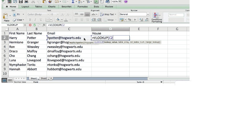
Lookup Value: The identical value you have in both spreadsheets. Choose the first value in your first spreadsheet. In Sprung's example that follows, this means the first email address on the list, or cell 2 (C2).

Table Array: The range of columns on Sheet 2 you're going to pull your data from, including the column of data identical to your lookup value (in our example, email addresses) in Sheet 1 as well as the column of data you're trying to copy to Sheet 1. In our example, this is "Sheet2!A:B." "A" means Column A in Sheet 2, which is the column in Sheet 2 where the data identical to our lookup value (email) in Sheet 1 is listed. The "B" means Column B, which contains the information that's only available in Sheet 2 that you want to translate to Sheet 1.

Column Number: The table array tells Excel where (which column) the new data you want to copy to Sheet 1 is located. In our example, this would be the "House" column, the second one in our table array, making it column number 2.

Range Lookup: Use FALSE to ensure you pull in only exact value matches.

- The formula with variables from Sprung's example below: 

=VLOOKUP(C2,Sheet2!A:B,2,FALSE)

(VLOOKUP is only left-to-right) Simpler to use and doesn't require selecting the entire table.